%load_ext autoreload
%autoreload 2

import xarray as xr
import xgcm
import matplotlib.pyplot as plt

Tutorial: analyzing finite-volume ocean model budgets with xbudget

This tutorial shows how to use xbudget to close and manipulate mass and tracer budgets in finite-volume.

Load example MOM6 dataset from Zenodo

from load_example_model_grid import load_MOM6_coarsened_diagnostics
grid = load_MOM6_coarsened_diagnostics()

File 'MOM6_global_example_diagnostics_zlevels_v0_0_6.nc' already exists at ../data/MOM6_global_example_diagnostics_zlevels_v0_0_6.nc. Skipping download.

Load budget metadata from preset MOM6 dictionary

import xbudget
recipe = xbudget.load_preset_budget(model="MOM6").copy()

We load in the file xbudget/recipes/MOM6.yaml, which comprehensively details the mass, heat, and salt budgets in MOM6, and how they can be evaluated using various combinations of diagnostics. In MOM6, most mass and tracer diagnostics are output as thickness tendencies and thickness-weighted tracer tendencies, respectively, and must be converted into density-weighted integrals over a finite-volume cell by multiplying by a seawater density and grid cell area.

For example, consider the structure of the heat budget:

xbudget.show_recipe(recipe, "heat")

xbudget recipe · heat

heatlambda=thetaosurface_lambda=tos

lhsΣ

Eulerian_tendency×

tracer_content_tendency_per_unit_area: opottemptend

area: areacello

advectionΣ

lateral×

sign: -1.

tracer_content_tendency_per_unit_area: T_advection_xy

area: areacello

interfacial×

sign: -1.

tracer_content_tendency_per_unit_area: Th_tendency_vert_remap

area: areacello

surface_ocean_flux_advective_negative_lhs×

sign: -1.

specific_heat_capacity: 3992.

lambda_mass: tos

thickness_tendency: boundary_forcing_h_tendency

density: 1035.

area: areacello

rhsΣ

diffusionΣ

lateral×

tracer_content_tendency_per_unit_area: opottemppmdiff

area: areacello

interfacial×

tracer_content_tendency_per_unit_area: opottempdiff

area: areacello

surface_exchange_flux×Σ

×product

tracer_content_tendency_per_unit_area: boundary_forcing_heat_tendency

area: areacello

Σsum

nonadvectiveΣ

latent×

tracer_content_tendency_per_unit_area: hflso

area: areacello

sensible×

tracer_content_tendency_per_unit_area: hfsso

area: areacello

longwave×

tracer_content_tendency_per_unit_area: rlntds

area: areacello

shortwave×

tracer_content_tendency_per_unit_area: rsdoabsorb

area: areacello

advective×

tracer_content_tendency_per_unit_area: heat_content_surfwater

area: areacello

surface_ocean_flux_advective_negative_rhs×

sign: -1.

specific_heat_capacity: 3992.

lambda_mass: tos

thickness_tendency: boundary_forcing_h_tendency

density: 1035.

area: areacello

bottom_flux×

tracer_content_tendency_per_unit_area: internal_heat_heat_tendency

area: areacello

frazil_ice×

tracer_content_tendency_per_unit_area: frazil_heat_tendency

area: areacello

The var: null entries in the dictionary denote where diagnostics are not directly available. In many cases, however, they can be reconstructed by taking the sum or product of available diagnostics.

We can use the xbudget.collect_budgets function to leverage the information in this metadata dictionary to fill in all of these gaps in the budget.

xbudget.collect_budgets(grid, recipe)
q = xbudget.BudgetQuery(grid, recipe)

Every reconstructed term is added to the original dataset (lazily), named after its path through the budget tree: the advection term under heat/lhs becomes heat_lhs_advection. Your metadata dictionary is left exactly as you wrote it.

BudgetQuery is how you ask what was built, without having to know the naming rule or search the dataset by eye.

q.aggregate()['heat']

{'lambda': 'thetao',
 'surface_lambda': 'tos',
 'lhs': {'Eulerian_tendency': 'heat_lhs_Eulerian_tendency',
  'advection': 'heat_lhs_advection',
  'surface_ocean_flux_advective_negative_lhs': 'heat_lhs_surface_ocean_flux_advective_negative_lhs'},
 'rhs': {'diffusion': 'heat_rhs_diffusion',
  'surface_exchange_flux': 'heat_rhs_surface_exchange_flux',
  'surface_ocean_flux_advective_negative_rhs': 'heat_rhs_surface_ocean_flux_advective_negative_rhs',
  'bottom_flux': 'heat_rhs_bottom_flux',
  'frazil_ice': 'heat_rhs_frazil_ice'}}

aggregate gives the high-level terms of each budget. To go the other way – from a term to the variable holding it – use q.var:

grid._ds[q.var("heat_lhs_advection")]

<xarray.DataArray 'heat_lhs_advection' (time: 1, z_l: 35, yh: 180, xh: 240)> Size: 12MB
dask.array<add, shape=(1, 35, 180, 240), dtype=float64, chunksize=(1, 35, 100, 100), chunktype=numpy.ndarray>
Coordinates:
    geolon     (yh, xh) float64 346kB dask.array<chunksize=(100, 100), meta=np.ndarray>
    lon        (yh, xh) float64 346kB dask.array<chunksize=(100, 100), meta=np.ndarray>
    geolat     (yh, xh) float64 346kB dask.array<chunksize=(100, 100), meta=np.ndarray>
    lat        (yh, xh) float64 346kB dask.array<chunksize=(100, 100), meta=np.ndarray>
    deptho     (yh, xh) float32 173kB dask.array<chunksize=(100, 100), meta=np.ndarray>
    wet        (yh, xh) float32 173kB dask.array<chunksize=(100, 100), meta=np.ndarray>
  * z_l        (z_l) float64 280B 2.5 10.0 20.0 32.5 ... 5.5e+03 6e+03 6.5e+03
  * time       (time) object 8B 2000-07-01 00:00:00
    areacello  (yh, xh) float64 346kB dask.array<chunksize=(100, 100), meta=np.ndarray>
  * xh         (xh) int64 2kB 0 1 2 3 4 5 6 7 ... 233 234 235 236 237 238 239
  * yh         (yh) int64 1kB 0 1 2 3 4 5 6 7 ... 173 174 175 176 177 178 179
Attributes:
    provenance:    ['heat_lhs_advection_lateral', 'heat_lhs_advection_interfa...
    xbudget_path:  ['heat', 'lhs', 'advection']
    xbudget_op:    sum

xarray.DataArray

'heat_lhs_advection'

• time: 1
• z_l: 35
• yh: 180
• xh: 240

• dask.array<chunksize=(1, 35, 100, 100), meta=np.ndarray>

  Array Chunk Bytes 11.54 MiB 2.67 MiB Shape (1, 35, 180, 240) (1, 35, 100, 100) Dask graph 6 chunks in 11 graph layers Data type float64 numpy.ndarray

• Coordinates: (11)
  • geolon
    (yh, xh)
    float64
    dask.array<chunksize=(100, 100), meta=np.ndarray>

    long_name :

    Longitude of tracer (T) points

    units :

    degrees_east

    cell_methods :

    time: point

    Array Chunk Bytes 337.50 kiB 78.12 kiB Shape (180, 240) (100, 100) Dask graph 6 chunks in 2 graph layers Data type float64 numpy.ndarray

  • lon
    (yh, xh)
    float64
    dask.array<chunksize=(100, 100), meta=np.ndarray>

    long_name :

    Longitude of tracer (T) points

    units :

    degrees_east

    cell_methods :

    time: point

    Array Chunk Bytes 337.50 kiB 78.12 kiB Shape (180, 240) (100, 100) Dask graph 6 chunks in 2 graph layers Data type float64 numpy.ndarray

  • geolat
    (yh, xh)
    float64
    dask.array<chunksize=(100, 100), meta=np.ndarray>

    long_name :

    Latitude of tracer (T) points

    units :

    degrees_north

    cell_methods :

    time: point

    Array Chunk Bytes 337.50 kiB 78.12 kiB Shape (180, 240) (100, 100) Dask graph 6 chunks in 2 graph layers Data type float64 numpy.ndarray

  • lat
    (yh, xh)
    float64
    dask.array<chunksize=(100, 100), meta=np.ndarray>

    long_name :

    Latitude of tracer (T) points

    units :

    degrees_north

    cell_methods :

    time: point

    Array Chunk Bytes 337.50 kiB 78.12 kiB Shape (180, 240) (100, 100) Dask graph 6 chunks in 2 graph layers Data type float64 numpy.ndarray

  • deptho
    (yh, xh)
    float32
    dask.array<chunksize=(100, 100), meta=np.ndarray>

    long_name :

    Sea Floor Depth

    units :

    m

    cell_methods :

    xh:mean yh:mean time:point

    cell_measures :

    area: areacello

    standard_name :

    sea_floor_depth_below_geoid

    Array Chunk Bytes 168.75 kiB 39.06 kiB Shape (180, 240) (100, 100) Dask graph 6 chunks in 2 graph layers Data type float32 numpy.ndarray

  • wet
    (yh, xh)
    float32
    dask.array<chunksize=(100, 100), meta=np.ndarray>

    long_name :

    0 if land, 1 if ocean at tracer points

    cell_methods :

    xh:mean yh:mean time:point

    cell_measures :

    area: areacello

    note :

    Can be between 0 and 1 if coarse cell includes both wet and dry sub-cells.

    Array Chunk Bytes 168.75 kiB 39.06 kiB Shape (180, 240) (100, 100) Dask graph 6 chunks in 2 graph layers Data type float32 numpy.ndarray

  • z_l
    (z_l)
    float64
    2.5 10.0 20.0 ... 6e+03 6.5e+03

    array([2.5000e+00, 1.0000e+01, 2.0000e+01, 3.2500e+01, 5.1250e+01, 7.5000e+01,
           1.0000e+02, 1.2500e+02, 1.5625e+02, 2.0000e+02, 2.5000e+02, 3.1250e+02,
           4.0000e+02, 5.0000e+02, 6.0000e+02, 7.0000e+02, 8.0000e+02, 9.0000e+02,
           1.0000e+03, 1.1000e+03, 1.2000e+03, 1.3000e+03, 1.4000e+03, 1.5375e+03,
           1.7500e+03, 2.0625e+03, 2.5000e+03, 3.0000e+03, 3.5000e+03, 4.0000e+03,
           4.5000e+03, 5.0000e+03, 5.5000e+03, 6.0000e+03, 6.5000e+03])

  • time
    (time)
    object
    2000-07-01 00:00:00

    long_name :

    historical time

    axis :

    T

    calendar_type :

    NOLEAP

    bounds :

    time_bnds

    cell_methods :

    time:mean

    array([cftime.DatetimeNoLeap(2000, 7, 1, 0, 0, 0, 0, has_year_zero=True)],
          dtype=object)

  • areacello
    (yh, xh)
    float64
    dask.array<chunksize=(100, 100), meta=np.ndarray>

    long_name :

    Ocean Grid-Cell Area

    units :

    m2

    cell_methods :

    area:sum yh:sum xh:sum time: point

    standard_name :

    cell_area

    note :

    We ignore land cells in partially wet cells when coarsening, so that tracer content can be accurately reconstructed by multiplying coarsened area-averaged tendencies by it. Fully wet (`wet==1.0`) and fully dry (`wet==0.0`) cells should be unaffected, and will just represent the total cell area. For the partially wet cells, total cell area can be derived from the ocean area by divding `areacello` by `wet`.

    Array Chunk Bytes 337.50 kiB 78.12 kiB Shape (180, 240) (100, 100) Dask graph 6 chunks in 2 graph layers Data type float64 numpy.ndarray

  • xh
    (xh)
    int64
    0 1 2 3 4 5 ... 235 236 237 238 239

    long_name :

    cell center x-index (nominally longitude)

    cell_methods :

    xh:point

    array([  0,   1,   2, ..., 237, 238, 239], shape=(240,))

  • yh
    (yh)
    int64
    0 1 2 3 4 5 ... 175 176 177 178 179

    long_name :

    cell center y-index (nominally latitude)

    cell_methods :

    yh:point

    array([  0,   1,   2,   3,   4,   5,   6,   7,   8,   9,  10,  11,  12,  13,
            14,  15,  16,  17,  18,  19,  20,  21,  22,  23,  24,  25,  26,  27,
            28,  29,  30,  31,  32,  33,  34,  35,  36,  37,  38,  39,  40,  41,
            42,  43,  44,  45,  46,  47,  48,  49,  50,  51,  52,  53,  54,  55,
            56,  57,  58,  59,  60,  61,  62,  63,  64,  65,  66,  67,  68,  69,
            70,  71,  72,  73,  74,  75,  76,  77,  78,  79,  80,  81,  82,  83,
            84,  85,  86,  87,  88,  89,  90,  91,  92,  93,  94,  95,  96,  97,
            98,  99, 100, 101, 102, 103, 104, 105, 106, 107, 108, 109, 110, 111,
           112, 113, 114, 115, 116, 117, 118, 119, 120, 121, 122, 123, 124, 125,
           126, 127, 128, 129, 130, 131, 132, 133, 134, 135, 136, 137, 138, 139,
           140, 141, 142, 143, 144, 145, 146, 147, 148, 149, 150, 151, 152, 153,
           154, 155, 156, 157, 158, 159, 160, 161, 162, 163, 164, 165, 166, 167,
           168, 169, 170, 171, 172, 173, 174, 175, 176, 177, 178, 179])

• Indexes: (4)
  • z_l
    PandasIndex

    PandasIndex(Index([   2.5,   10.0,   20.0,   32.5,  51.25,   75.0,  100.0,  125.0, 156.25,
            200.0,  250.0,  312.5,  400.0,  500.0,  600.0,  700.0,  800.0,  900.0,
           1000.0, 1100.0, 1200.0, 1300.0, 1400.0, 1537.5, 1750.0, 2062.5, 2500.0,
           3000.0, 3500.0, 4000.0, 4500.0, 5000.0, 5500.0, 6000.0, 6500.0],
          dtype='float64', name='z_l'))

  • time
    PandasIndex

    PandasIndex(CFTimeIndex([2000-07-01 00:00:00],
                dtype='object', length=1, calendar='noleap', freq=None))

  • xh
    PandasIndex

    PandasIndex(Index([  0,   1,   2,   3,   4,   5,   6,   7,   8,   9,
           ...
           230, 231, 232, 233, 234, 235, 236, 237, 238, 239],
          dtype='int64', name='xh', length=240))

  • yh
    PandasIndex

    PandasIndex(Index([  0,   1,   2,   3,   4,   5,   6,   7,   8,   9,
           ...
           170, 171, 172, 173, 174, 175, 176, 177, 178, 179],
          dtype='int64', name='yh', length=180))

• Attributes: (3)

  provenance :

  ['heat_lhs_advection_lateral', 'heat_lhs_advection_interfacial']

  xbudget_path :

  ['heat', 'lhs', 'advection']

  xbudget_op :

  sum

If the variable is not immediately available as a diagnostic–but instead derived from other diagnostics–the provenance attribute points to the origin of the variable.

Note that q.var above and q.get_vars below are asking about the same variable: get_vars additionally reports the terms that feed into it. For variables that are the sum or product of other terms, that list is the decomposition:

q.get_vars("heat_lhs_advection")

{'var': 'heat_lhs_advection',
 'sum': ['heat_lhs_advection_lateral', 'heat_lhs_advection_interfacial']}

The terms from which the variable is derived are not necessarily other xr.DataArray objects–they can also be constant numbers.

q.get_vars("heat_lhs_surface_ocean_flux_advective_negative_lhs")

{'var': 'heat_lhs_surface_ocean_flux_advective_negative_lhs',
 'product': [-1.0,
  3992.0,
  'tos',
  'boundary_forcing_h_tendency',
  1035.0,
  'areacello']}

get_vars takes either a single address or a list of them, and a raw diagnostic name works too (it reports which terms use it):

q.get_vars(["heat_lhs", "heat_rhs_diffusion", "boundary_forcing_heat_tendency"])

[{'var': 'heat_lhs',
  'sum': ['heat_lhs_Eulerian_tendency',
   'heat_lhs_advection',
   'heat_lhs_surface_ocean_flux_advective_negative_lhs']},
 {'var': 'heat_rhs_diffusion',
  'sum': ['heat_rhs_diffusion_lateral', 'heat_rhs_diffusion_interfacial']},
 {'var': 'boundary_forcing_heat_tendency',
  'referenced_by': [('heat', 'rhs', 'surface_exchange_flux')]}]

Verification that the budgets close

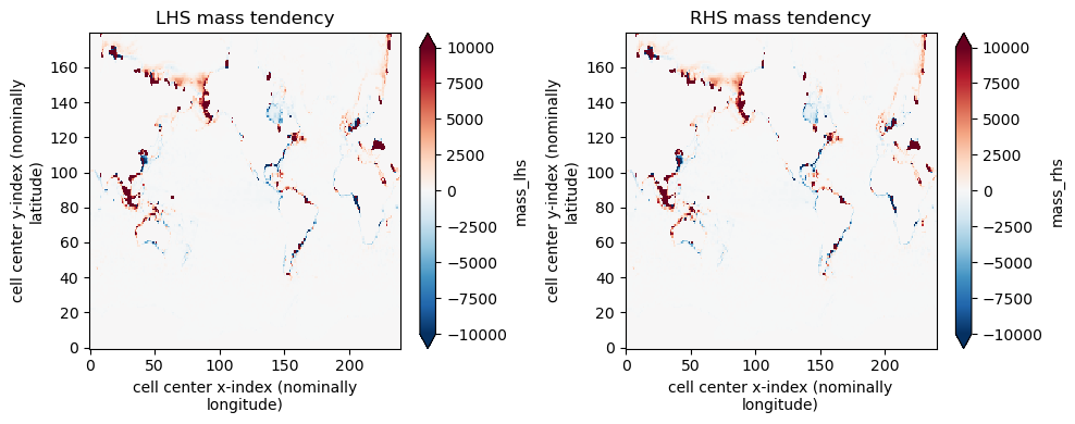
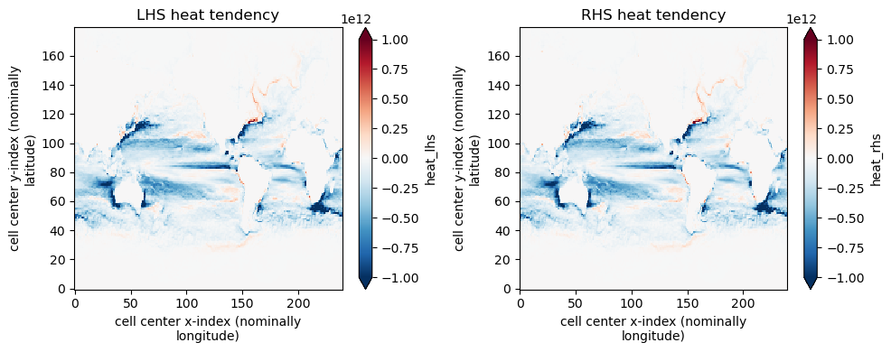
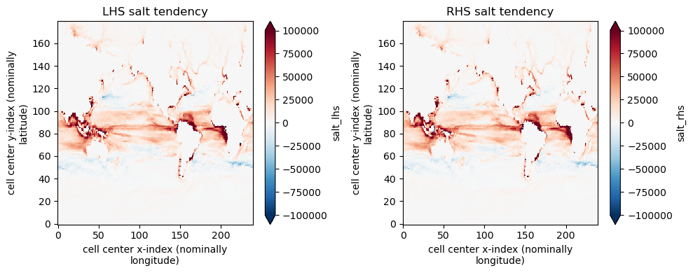
We compare the left-hand-side (LHS) tendency terms against the sum of all of the right-hand-side (RHS) terms.

for eq, vmax in zip(["mass", "heat", "salt"], [1.e4, 1e12, 1.e5]):
    plt.figure(figsize=(10, 4))

    plt.subplot(1,2,1)
    pc = grid._ds[q.var(f"{eq}_lhs")].isel(z_l = 0).isel(time=0).plot(vmin=-vmax, vmax=vmax, cmap="RdBu_r")
    plt.title(f"LHS {eq} tendency")

    plt.subplot(1,2,2)
    pc = grid._ds[q.var(f"{eq}_rhs")].isel(z_l = 0).isel(time=0).plot(vmin=-vmax, vmax=vmax, cmap="RdBu_r")
    plt.title(f"RHS {eq} tendency")

    plt.tight_layout()

Decompose RHS budget terms with xbudget

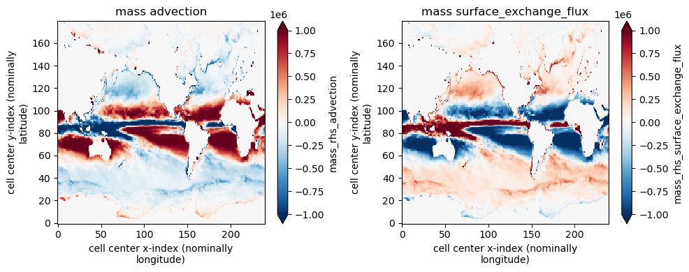
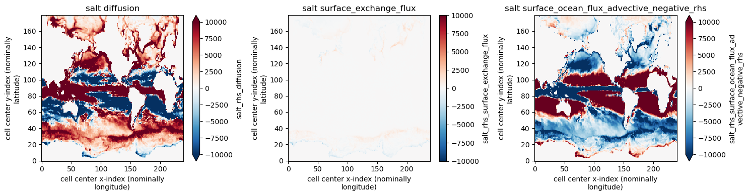
Since the full budget is relatively clunky and can be decomposed in a number of different ways, we include helper functions for collecting all of the high-level terms and optionally dissaggreating terms of interest:

# Default high-level aggregate budget
simple_budgets = q.aggregate()
simple_budgets

{'mass': {'lambda': 'density',
  'thickness': 'thkcello',
  'lhs': {'Eulerian_tendency': 'mass_lhs_Eulerian_tendency'},
  'rhs': {'advection': 'mass_rhs_advection',
   'surface_exchange_flux': 'mass_rhs_surface_exchange_flux'}},
 'heat': {'lambda': 'thetao',
  'surface_lambda': 'tos',
  'lhs': {'Eulerian_tendency': 'heat_lhs_Eulerian_tendency',
   'advection': 'heat_lhs_advection',
   'surface_ocean_flux_advective_negative_lhs': 'heat_lhs_surface_ocean_flux_advective_negative_lhs'},
  'rhs': {'diffusion': 'heat_rhs_diffusion',
   'surface_exchange_flux': 'heat_rhs_surface_exchange_flux',
   'surface_ocean_flux_advective_negative_rhs': 'heat_rhs_surface_ocean_flux_advective_negative_rhs',
   'bottom_flux': 'heat_rhs_bottom_flux',
   'frazil_ice': 'heat_rhs_frazil_ice'}},
 'salt': {'lambda': 'so',
  'surface_lambda': 'sos',
  'lhs': {'Eulerian_tendency': 'salt_lhs_Eulerian_tendency',
   'advection': 'salt_lhs_advection',
   'surface_ocean_flux_advective_negative_lhs': 'salt_lhs_surface_ocean_flux_advective_negative_lhs'},
  'rhs': {'diffusion': 'salt_rhs_diffusion',
   'surface_exchange_flux': 'salt_rhs_surface_exchange_flux',
   'surface_ocean_flux_advective_negative_rhs': 'salt_rhs_surface_ocean_flux_advective_negative_rhs'}}}

vmax = 1.e-4

for eq, vmax in zip(["mass", "heat", "salt"], [1.e6, 1e12, 1e4]):
    N = len(simple_budgets[eq]['rhs'])
    plt.figure(figsize=(5*N, 4))
    for i, (k,v) in enumerate(simple_budgets[eq]['rhs'].items(), start=1):
        plt.subplot(1,N, i)
        if "z_l" in grid._ds[v].dims:
            grid._ds[v].isel(z_l = 0).isel(time=0).plot(vmin=-vmax, vmax=vmax, cmap="RdBu_r")
        else:
            grid._ds[v].isel(time=0).plot(vmin=-vmax, vmax=vmax, cmap="RdBu_r")
        plt.title(f"{eq} {k}")

    plt.tight_layout()

Custom budget decompositions

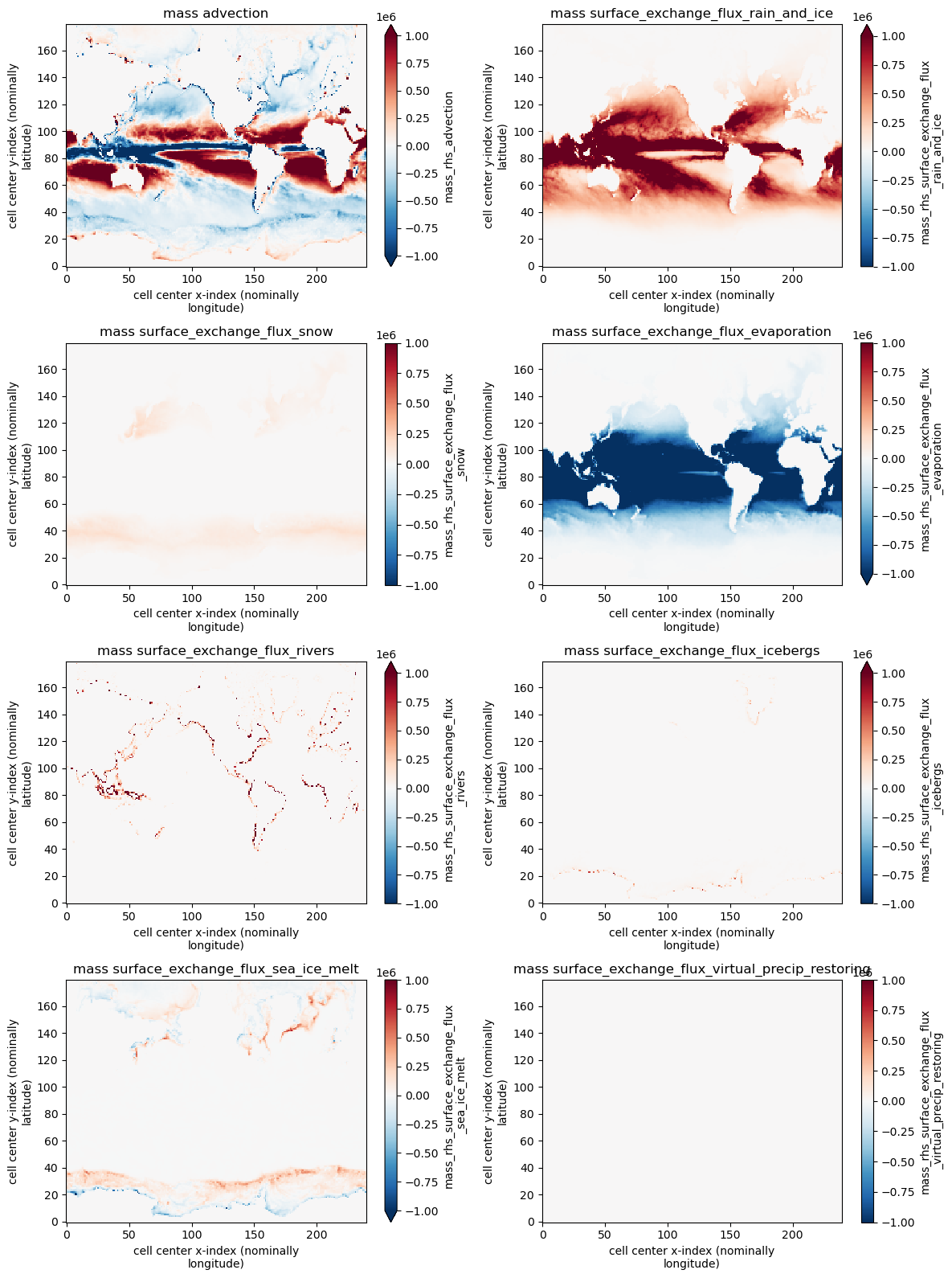
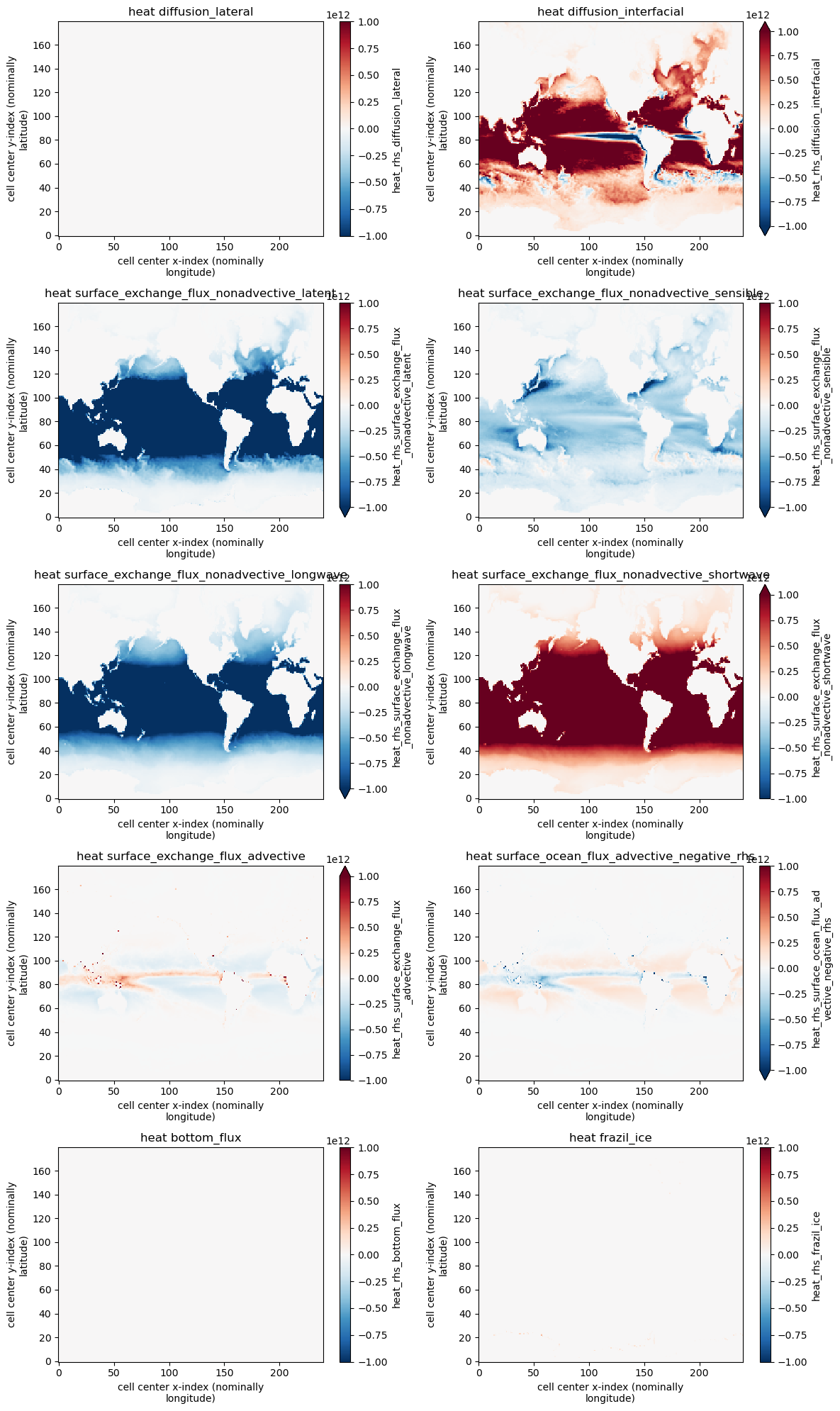
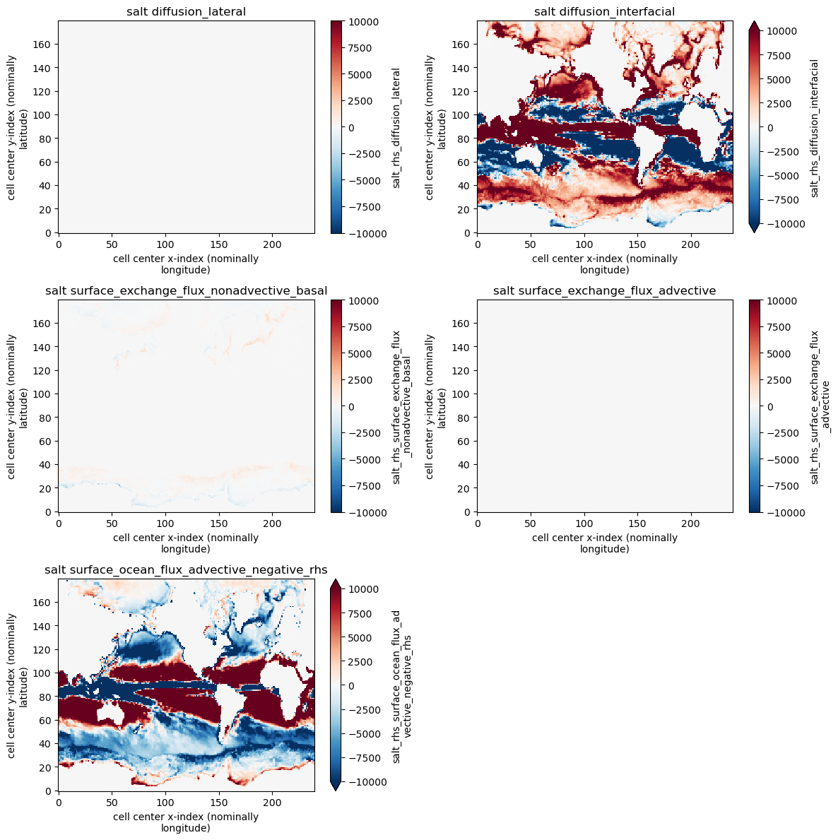
Suppose we want to have a better understanding of the processes driving both the surface_flux terms and interior diffusion terms. We can simply pass the list of these process names to the decompose keyword argument. We can also further breakdown the nonadvective part of the surface_flux term.

decomposed_budgets = q.aggregate(decompose=["surface_exchange_flux", "nonadvective", "diffusion"])
decomposed_budgets

{'mass': {'lambda': 'density',
  'thickness': 'thkcello',
  'lhs': {'Eulerian_tendency': 'mass_lhs_Eulerian_tendency'},
  'rhs': {'advection': 'mass_rhs_advection',
   'surface_exchange_flux_rain_and_ice': 'mass_rhs_surface_exchange_flux_rain_and_ice',
   'surface_exchange_flux_snow': 'mass_rhs_surface_exchange_flux_snow',
   'surface_exchange_flux_evaporation': 'mass_rhs_surface_exchange_flux_evaporation',
   'surface_exchange_flux_rivers': 'mass_rhs_surface_exchange_flux_rivers',
   'surface_exchange_flux_icebergs': 'mass_rhs_surface_exchange_flux_icebergs',
   'surface_exchange_flux_sea_ice_melt': 'mass_rhs_surface_exchange_flux_sea_ice_melt',
   'surface_exchange_flux_virtual_precip_restoring': 'mass_rhs_surface_exchange_flux_virtual_precip_restoring'}},
 'heat': {'lambda': 'thetao',
  'surface_lambda': 'tos',
  'lhs': {'Eulerian_tendency': 'heat_lhs_Eulerian_tendency',
   'advection': 'heat_lhs_advection',
   'surface_ocean_flux_advective_negative_lhs': 'heat_lhs_surface_ocean_flux_advective_negative_lhs'},
  'rhs': {'diffusion_lateral': 'heat_rhs_diffusion_lateral',
   'diffusion_interfacial': 'heat_rhs_diffusion_interfacial',
   'surface_exchange_flux_nonadvective_latent': 'heat_rhs_surface_exchange_flux_nonadvective_latent',
   'surface_exchange_flux_nonadvective_sensible': 'heat_rhs_surface_exchange_flux_nonadvective_sensible',
   'surface_exchange_flux_nonadvective_longwave': 'heat_rhs_surface_exchange_flux_nonadvective_longwave',
   'surface_exchange_flux_nonadvective_shortwave': 'heat_rhs_surface_exchange_flux_nonadvective_shortwave',
   'surface_exchange_flux_advective': 'heat_rhs_surface_exchange_flux_advective',
   'surface_ocean_flux_advective_negative_rhs': 'heat_rhs_surface_ocean_flux_advective_negative_rhs',
   'bottom_flux': 'heat_rhs_bottom_flux',
   'frazil_ice': 'heat_rhs_frazil_ice'}},
 'salt': {'lambda': 'so',
  'surface_lambda': 'sos',
  'lhs': {'Eulerian_tendency': 'salt_lhs_Eulerian_tendency',
   'advection': 'salt_lhs_advection',
   'surface_ocean_flux_advective_negative_lhs': 'salt_lhs_surface_ocean_flux_advective_negative_lhs'},
  'rhs': {'diffusion_lateral': 'salt_rhs_diffusion_lateral',
   'diffusion_interfacial': 'salt_rhs_diffusion_interfacial',
   'surface_exchange_flux_nonadvective_basal': 'salt_rhs_surface_exchange_flux_nonadvective_basal',
   'surface_exchange_flux_advective': 'salt_rhs_surface_exchange_flux_advective',
   'surface_ocean_flux_advective_negative_rhs': 'salt_rhs_surface_ocean_flux_advective_negative_rhs'}}}

decomposed_budgets[eq]['rhs']

{'diffusion_lateral': 'salt_rhs_diffusion_lateral',
 'diffusion_interfacial': 'salt_rhs_diffusion_interfacial',
 'surface_exchange_flux_nonadvective_basal': 'salt_rhs_surface_exchange_flux_nonadvective_basal',
 'surface_exchange_flux_advective': 'salt_rhs_surface_exchange_flux_advective',
 'surface_ocean_flux_advective_negative_rhs': 'salt_rhs_surface_ocean_flux_advective_negative_rhs'}

vmax = 1.e-4
import numpy as np

for eq, vmax in zip(["mass", "heat", "salt"], [1e6, 1e12, 1e4]):
    nrow = np.int64(np.ceil(len(decomposed_budgets[eq]['rhs'])/2))
    plt.figure(figsize=(12, nrow*4))
    for i, (k,v) in enumerate(decomposed_budgets[eq]['rhs'].items(), start=1):
        plt.subplot(nrow, 2, i)
        if "z_l" in grid._ds[v].dims:
            grid._ds[v].isel(z_l = 0).isel(time=0).plot(vmin=-vmax, vmax=vmax, cmap="RdBu_r")
        else:
            grid._ds[v].isel(time=0).plot(vmin=-vmax, vmax=vmax, cmap="RdBu_r")
        plt.title(f"{eq} {k}")

    plt.tight_layout()
    plt.show()