%load_ext autoreload
%autoreload 2

import xarray as xr
import numpy as np
from scipy.interpolate import griddata
import xgcm
import matplotlib.pyplot as plt
import xbudget

from load_example_ecco_grid import *
from eccov4r4_budget_diagnostics import *
from xbudget.llc90 import *
print("xarray:",  xr.__version__)
print("xgcm:", xgcm.__version__)

xarray: 2026.2.0
xgcm: 0.9.0

Tutorial: ECCO V4r4 example

This tutorial gives a compact introduction to the ECCO V4r4 budget diagnostics and shows how to use xbudget to assemble and verify mass, heat, and salt budgets on the LLC grid.

Load example ECCO V4r4 dataset from Zenodo

The example loader returns an xgcm.Grid object together with the underlying ECCO dataset in grid._ds.

grid = load_ECCOV4r4_coarsened_diagnostics() # this takes about 7 minutes

# Build a time-step coordinate and a cell-volume metric used repeatedly below.
dt = grid._ds["time_bounds"].diff("time_bounds").rename({"time_bounds":"time"})

grid._ds = grid._ds.assign_coords(
    {"dt":("time", dt.dt.total_seconds().values),
    "volcello": (grid._ds["drF"] * grid._ds["hFacC"]) * grid._ds["rA"]
    }
)

File 'ECCO_budget_terms.nc' already exists at ../data/ECCO_budget_terms.nc. Skipping download.

Preprocess standard ECCO diagnostics

The ECCO V4r4 fields hosted on PO.DAAC contain the ingredients needed to close native-grid mass, heat, and salt budgets, but a few terms need to be reorganized before they match the bookkeeping expected by xbudget. In particular, some diagnostics combine interior and boundary contributions, while others separate penetrative and non-penetrative surface forcing.

def zero_top_layer(ds, varname = "", zdim = "k_l"):
    # Remove the surface layer contribution when a diagnostic should only represent interior transport.
    return xr.where(ds[f"{zdim}"] != ds[f"{zdim}"].isel({f"{zdim}":0}),ds[varname].copy(),0.0,)
def make_flux_3d(ds, varname = "", zdim = "k"):
    # Broadcast a surface flux into a 3D array that only occupies the top model layer.
    k  = ds[f"{zdim}"]
    return xr.where(k == k.isel({f"{zdim}":0}), ds[varname].copy().expand_dims({f"{zdim}":k}),0.0,)

# Assemble ECCO heat-flux terms into the budget components expected by xbudget.
grid._ds["geothermal_heat_flux_convergence"] = eccov4r4_geothermal_heat_flux_tendency(grid._ds)
grid._ds["pen_boundary_forcing_heat_tendency"] = eccov4r4_penetrative_heat_flux_tendency(grid._ds)
grid._ds["nonpen_boundary_forcing_heat_tendency"] = eccov4r4_nonpenetrative_heat_flux_tendency(grid._ds)
grid._ds["boundary_forcing_heat_tendency"] = grid._ds["pen_boundary_forcing_heat_tendency"] + grid._ds["nonpen_boundary_forcing_heat_tendency"]

# Put the sea-ice salt exchange and salt-plume tendency onto the same vertical grid.
SFLUX = grid._ds["SFLUX"].assign_coords(k=0).expand_dims(dim='k',axis=1) # sea-ice salt exchange
grid._ds["boundary_forcing_salt_tendency"] = xr.concat([SFLUX+grid._ds["oceSPtnd"],grid._ds["oceSPtnd"].isel(k=slice(1,None))], dim='k') # combine surface salt flux and plume tendency

# Separate interior vertical transport from the freshwater boundary forcing term.
grid._ds["WVELMASS_interior"] = zero_top_layer(grid._ds, varname = "WVELMASS", zdim = "k_l") #
grid._ds["boundary_forcing_volume_tendency"] = make_flux_3d(grid._ds, varname = "oceFWflx", zdim = "k")

# Rechunk once before calling xbudget so later difference and convergence steps stay tractable.
grid._ds = grid._ds.chunk({"tile":2, "i":50, "j":50, "i_g":50, "j_g":50, "k": 10}).fillna(0.0)
# to-do: add comparable chunking inside the difference and convergence routines

Load budget metadata from the ECCO preset dictionary

This preset tells xbudget which variables belong on the left-hand side, which belong on the right-hand side, and how derived budget terms should be combined.

# Load the preset metadata dictionary and let xbudget attach the derived budget terms.
xbudget_dict = xbudget.load_preset_budget(model="ECCOV4r4_native").copy()
xbudget.collect_budgets(grid, xbudget_dict,allow_rechunk= True)
# Aggregate the full metadata tree into a simpler budget summary for inspection.
simple_budgets = xbudget.aggregate(xbudget_dict)
simple_budgets

{'mass': {'lambda': 'density',
  'thickness': 'thkcello',
  'lhs': {'Eulerian_tendency': 'mass_lhs_sum_Eulerian_tendency'},
  'rhs': {'advection': 'mass_rhs_sum_advection',
   'surface_exchange_flux': 'mass_rhs_sum_surface_exchange_flux'}},
 'heat': {'lambda': 'THETA',
  'lhs': {'Eulerian_tendency': 'heat_lhs_sum_Eulerian_tendency'},
  'rhs': {'advection': 'heat_rhs_sum_advection',
   'diffusion': 'heat_rhs_sum_diffusion',
   'surface_exchange_flux': 'heat_rhs_sum_surface_exchange_flux',
   'bottom_flux': 'heat_rhs_sum_bottom_flux'}},
 'salt': {'lambda': 'SALT',
  'lhs': {'Eulerian_tendency': 'salt_lhs_sum_Eulerian_tendency'},
  'rhs': {'advection': 'salt_rhs_sum_advection',
   'diffusion': 'salt_rhs_sum_diffusion',
   'surface_exchange_flux': 'salt_rhs_sum_surface_exchange_flux'}}}

Verify that the budgets close

The checks below compare the left-hand-side (LHS) storage tendency against the diagnosed sum of the right-hand-side (RHS) source, sink, and flux-convergence terms. We look at both spatial patterns and globally averaged time series. Because ECCO uses the LLC grid, the maps are first remapped to a regular latitude-longitude grid for quick visualization.

Refer to MOM6_budget_examples_mass_heat_salt.ipynb for a more detailed explanation of the xbudget workflow.

def plot_interpolated_ecco(fig, ax, ds, vmin=0, vmax=30, cmap="coolwarm"):
    # Build a simple regular lat-lon target grid for quick visual comparison.
    target_lon = np.arange(-180, 180, 1)
    target_lat = np.arange(-90, 90, 1)
    lon_grid, lat_grid = np.meshgrid(target_lon, target_lat)

    # Flatten the LLC field into point/value pairs for interpolation.
    points = np.column_stack((ds.XC.values.ravel(), ds.YC.values.ravel()))
    values = ds.values.ravel()

    # Use nearest-neighbor remapping to preserve the native diagnostic values.
    interpolated_data = griddata(points, values, (lon_grid, lat_grid), method='nearest')

    # Plot the remapped field.
    cb = ax.pcolormesh(lon_grid, lat_grid, interpolated_data,
                       vmin=vmin, vmax=vmax, cmap=cmap)

    return cb

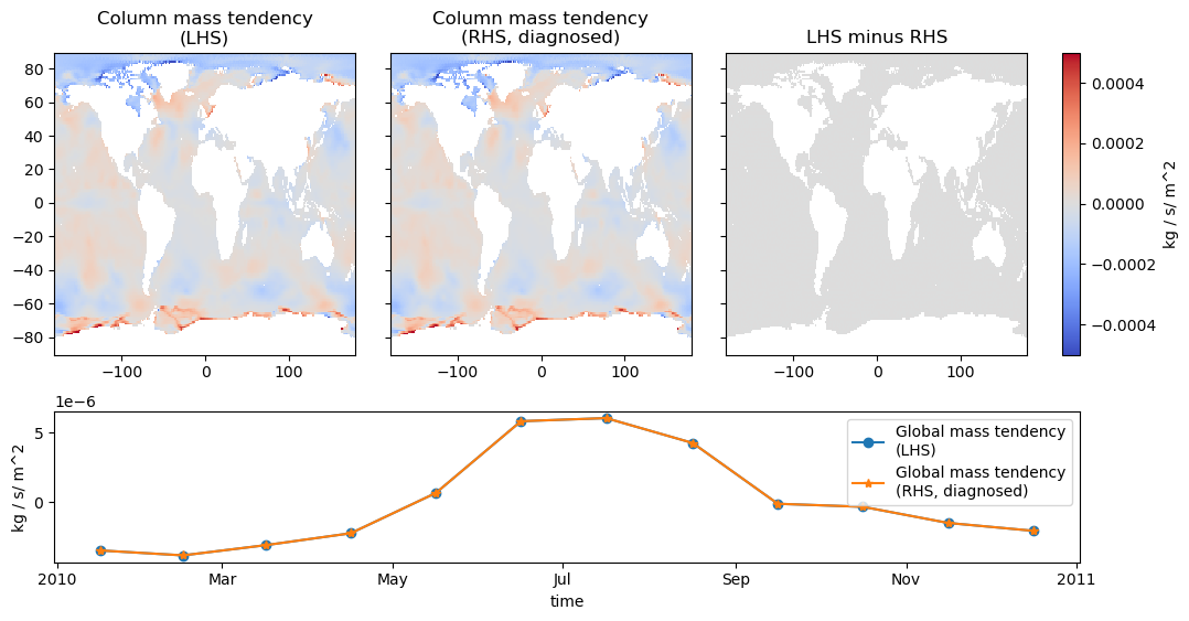
Volume budgets

This first check verifies that the vertically integrated volume tendency is balanced by the diagnosed transport and boundary-forcing terms.

fig = plt.figure(figsize=(12, 6))
gs = fig.add_gridspec(2, 4, width_ratios=[1, 1, 1,  0.06], height_ratios=[1, 0.5], hspace=0.25, wspace=0.15)

ax0 = fig.add_subplot(gs[0, 0])
ax1 = fig.add_subplot(gs[0, 1], sharey=ax0); ax1.tick_params(labelleft=False)
ax2 = fig.add_subplot(gs[0, 2], sharey=ax0); ax2.tick_params(labelleft=False)
cax = fig.add_subplot(gs[0, 3])
ax_bottom = fig.add_subplot(gs[1, :])

# Restrict horizontal area to wet points before forming column integrals.
area = grid._ds["rA"].where(grid._ds["Depth"] > 0.0)

# Convert native volume-integrated tendencies into column tendencies per unit area.
lhs_tendency = (grid._ds[xbudget.get_vars(xbudget_dict, "mass_lhs")["var"]] / area).sum("k") # convert from kg/s to kg / s/ m^2
lhs_tendency = lhs_tendency.where(np.abs(lhs_tendency) > 0.0)

rhs_tendency = (grid._ds[xbudget.get_vars(xbudget_dict, "mass_rhs_sum")["var"]] / area).sum("k")
rhs_tendency = rhs_tendency.where(np.abs(rhs_tendency) > 0.0)

# Residual should be small if the budget closes.
tendency_difference = lhs_tendency - rhs_tendency

vmax = 5e-4
plot_interpolated_ecco(fig, ax0, lhs_tendency.isel(time=0), vmin=-vmax, vmax=vmax); ax0.set_title("Column mass tendency\n(LHS)")
plot_interpolated_ecco(fig, ax1, rhs_tendency.isel(time=0), vmin=-vmax, vmax=vmax); ax1.set_title("Column mass tendency\n(RHS, diagnosed)")
cb = plot_interpolated_ecco(fig, ax2, tendency_difference.isel(time=0), vmin=-vmax, vmax=vmax); ax2.set_title("LHS minus RHS")
fig.colorbar(cb, cax=cax, orientation="vertical", label = "kg / s/ m^2")

# Area-weighted global means summarize the closure error over time.
((lhs_tendency * area) / area.sum()).sum(["tile", "i", "j"]).plot(ax = ax_bottom, marker = "o", label = "Global mass tendency\n(LHS)")
((rhs_tendency * area) / area.sum()).sum(["tile", "i", "j"]).plot(ax = ax_bottom, marker = "*", label = "Global mass tendency\n(RHS, diagnosed)")
ax_bottom.set_ylabel("kg / s/ m^2")
ax_bottom.legend()

<matplotlib.legend.Legend at 0x326af3fb0>

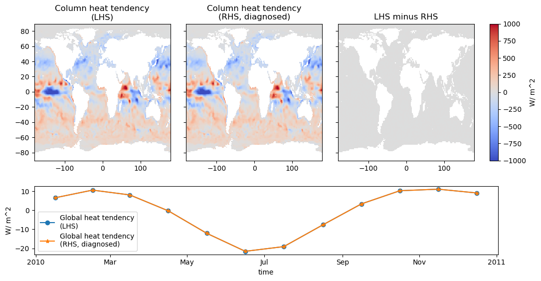
Heat budgets

This check compares the column-integrated heat tendency against the assembled surface and transport contributions.

fig = plt.figure(figsize=(12, 6))
gs = fig.add_gridspec(2, 4, width_ratios=[1, 1, 1,  0.06], height_ratios=[1, 0.5], hspace=0.25, wspace=0.15)

ax0 = fig.add_subplot(gs[0, 0])
ax1 = fig.add_subplot(gs[0, 1], sharey=ax0); ax1.tick_params(labelleft=False)
ax2 = fig.add_subplot(gs[0, 2], sharey=ax0); ax2.tick_params(labelleft=False)
cax = fig.add_subplot(gs[0, 3])
ax_bottom = fig.add_subplot(gs[1, :])

# Restrict horizontal area to wet points before forming column integrals.
area = grid._ds["rA"].where(grid._ds["Depth"] > 0.0)

# Convert native volume-integrated heat tendencies into column tendencies per unit area.
lhs_tendency = (grid._ds[xbudget.get_vars(xbudget_dict, "heat_lhs")['var']] / area).sum("k") # convert from J/s to W/m^2
lhs_tendency = lhs_tendency.where(np.abs(lhs_tendency) > 0.0)

rhs_tendency = (grid._ds[xbudget.get_vars(xbudget_dict, "heat_rhs")['var']] / area).sum("k")
rhs_tendency = rhs_tendency.where(np.abs(rhs_tendency) > 0.0)

# Residual should be small if the budget closes.
tendency_difference = lhs_tendency - rhs_tendency

vmax = 1000
plot_interpolated_ecco(fig, ax0, lhs_tendency.isel(time=0), vmin=-vmax, vmax=vmax); ax0.set_title("Column heat tendency\n(LHS)")
plot_interpolated_ecco(fig, ax1, rhs_tendency.isel(time=0), vmin=-vmax, vmax=vmax); ax1.set_title("Column heat tendency\n(RHS, diagnosed)")
cb = plot_interpolated_ecco(fig, ax2, tendency_difference.isel(time=0), vmin=-vmax, vmax=vmax); ax2.set_title("LHS minus RHS")
fig.colorbar(cb, cax=cax, orientation="vertical", label = "W/ m^2")

# Area-weighted global means summarize the closure error over time.
((lhs_tendency * area) / area.sum()).sum(["tile", "i", "j"]).plot(ax = ax_bottom, marker = "o", label = "Global heat tendency\n(LHS)")
((rhs_tendency * area) / area.sum()).sum(["tile", "i", "j"]).plot(ax = ax_bottom, marker = "*", label = "Global heat tendency\n(RHS, diagnosed)")
ax_bottom.set_ylabel("W/ m^2")
ax_bottom.legend()

<matplotlib.legend.Legend at 0x326c34f20>

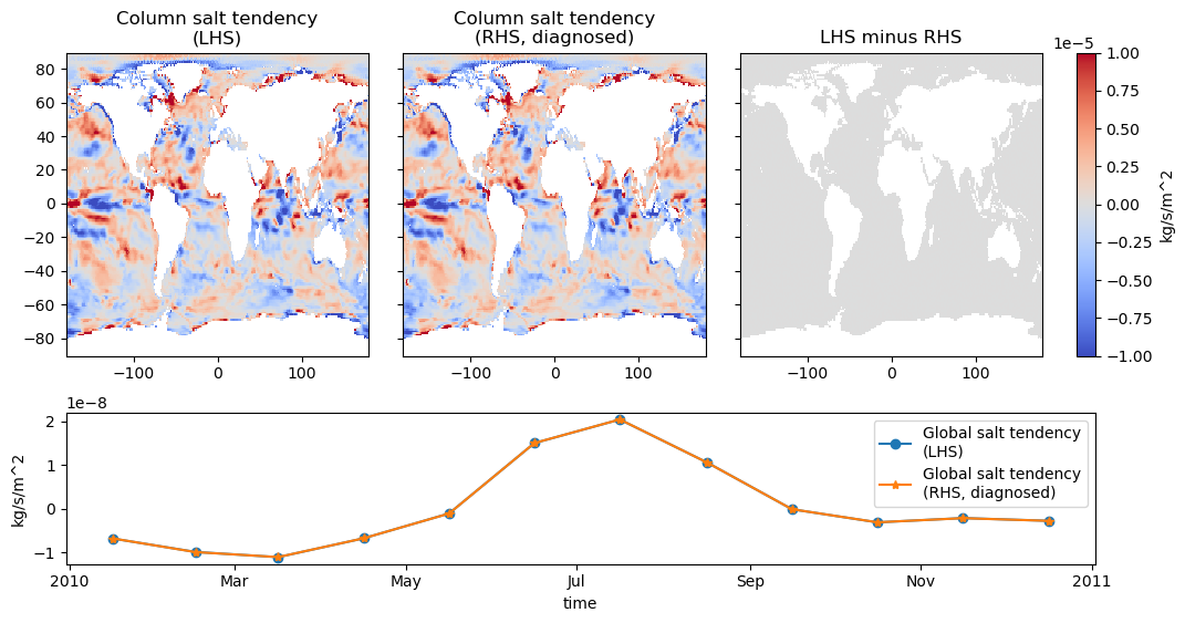
Salt budgets

This final check compares the column-integrated salt tendency against the diagnosed salt sources, sinks, and transport terms.

fig = plt.figure(figsize=(12, 6))
gs = fig.add_gridspec(2, 4, width_ratios=[1, 1, 1,  0.06], height_ratios=[1, 0.5], hspace=0.25, wspace=0.15)

ax0 = fig.add_subplot(gs[0, 0])
ax1 = fig.add_subplot(gs[0, 1], sharey=ax0); ax1.tick_params(labelleft=False)
ax2 = fig.add_subplot(gs[0, 2], sharey=ax0); ax2.tick_params(labelleft=False)
cax = fig.add_subplot(gs[0, 3])
ax_bottom = fig.add_subplot(gs[1, :])

# Restrict horizontal area to wet points before forming column integrals.
area = grid._ds["rA"].where(grid._ds["Depth"] > 0.0)

# Convert native volume-integrated salt tendencies into column tendencies per unit area.
lhs_tendency = (grid._ds[xbudget.get_vars(xbudget_dict, "salt_lhs")['var']] / area).sum("k") # convert from kg/s to kg/s/m^2
lhs_tendency = lhs_tendency.where(np.abs(lhs_tendency) > 0.0)

rhs_tendency = (grid._ds[xbudget.get_vars(xbudget_dict, "salt_rhs")['var']] / area).sum("k")
rhs_tendency = rhs_tendency.where(np.abs(rhs_tendency) > 0.0)

# Residual should be small if the budget closes.
tendency_difference = lhs_tendency - rhs_tendency

vmax = 1e-5
plot_interpolated_ecco(fig, ax0, lhs_tendency.isel(time=0), vmin=-vmax, vmax=vmax); ax0.set_title("Column salt tendency\n(LHS)")
plot_interpolated_ecco(fig, ax1, rhs_tendency.isel(time=0), vmin=-vmax, vmax=vmax); ax1.set_title("Column salt tendency\n(RHS, diagnosed)")
cb = plot_interpolated_ecco(fig, ax2, tendency_difference.isel(time=0), vmin=-vmax, vmax=vmax); ax2.set_title("LHS minus RHS")
fig.colorbar(cb, cax=cax, orientation="vertical", label = "kg/s/m^2")

# Area-weighted global means summarize the closure error over time.
((lhs_tendency * area) / area.sum()).sum(["tile", "i", "j"]).plot(ax = ax_bottom, marker = "o", label = "Global salt tendency\n(LHS)")
((rhs_tendency * area) / area.sum()).sum(["tile", "i", "j"]).plot(ax = ax_bottom, marker = "*", label = "Global salt tendency\n(RHS, diagnosed)")
ax_bottom.set_ylabel("kg/s/m^2")
ax_bottom.legend()

<matplotlib.legend.Legend at 0x35f79cf80>